Bulk ordering with cloud-aware selection
Placing a large archive order — hundreds or thousands of areas, each possibly at several dates — is not the single-area flow repeated N times. Choosing captures by hand does not scale, and the obvious automation (sort by the vendor’s cloud percentage, take the top result) buys the wrong imagery.
This guide covers the operations that make it tractable, with a worked example measured end to end on live archive data.
| Step | Operation | Side-effect | Scope |
|---|---|---|---|
| Find candidates | catalog.search | read | catalog:read |
| Choose the set | catalog.clear_coverage.plan | compute | catalog:read |
| Portfolio view | catalog.clear_coverage.campaign | compute | catalog:read |
| Preview price | orders.archive.estimate | read | orders:read |
| Place order | orders.archive.place | spend | orders:write |
Only the last step spends anything. plan and campaign are compute — you can run
them as often as you like while tuning thresholds.
Why cloud percentage is the wrong sort key
Two independent reasons, and the second surprises people more than the first.
The vendor’s cloud figure describes a whole scene, not your area. It is usually accurate — it just isn’t about you. A capture reported at 0% cloud can deliver a quarter of your area; one reported at 30% can deliver all of it. The scene is far larger than most areas of interest, so where the cloud sits matters more than how much there is.
Most areas need more than one capture anyway. A 0.5 m optical scene covers roughly 230 km². Any area larger than that needs a set, and the question stops being “which capture is best?” and becomes “which combination covers my area?“.
catalog.clear_coverage.plan answers the second question. It measures how much of
your area each candidate actually delivers clear of cloud and shadow, then selects the
smallest set that covers it — and tells you what that set will cost.
Do not filter on cloud when searching
The most important line in this guide. Send cloudCoverage: { "LTE": 100 }.
Filtering candidates on the vendor’s scene-wide percentage discards exactly the captures the planner exists to rescue, before it ever sees them. Let the planner measure them and reject them on evidence.
A worked example
A 698 km² area in Western Australia. catalog.search returned 23 candidates,
all 0.5 m optical. Here is the outcome before any of the detail — the same area, the
same scale, real pixels from the vendor’s own browse imagery:

The best capture in the archive covers a corner. The set the API returns fills the area, and costs the same.
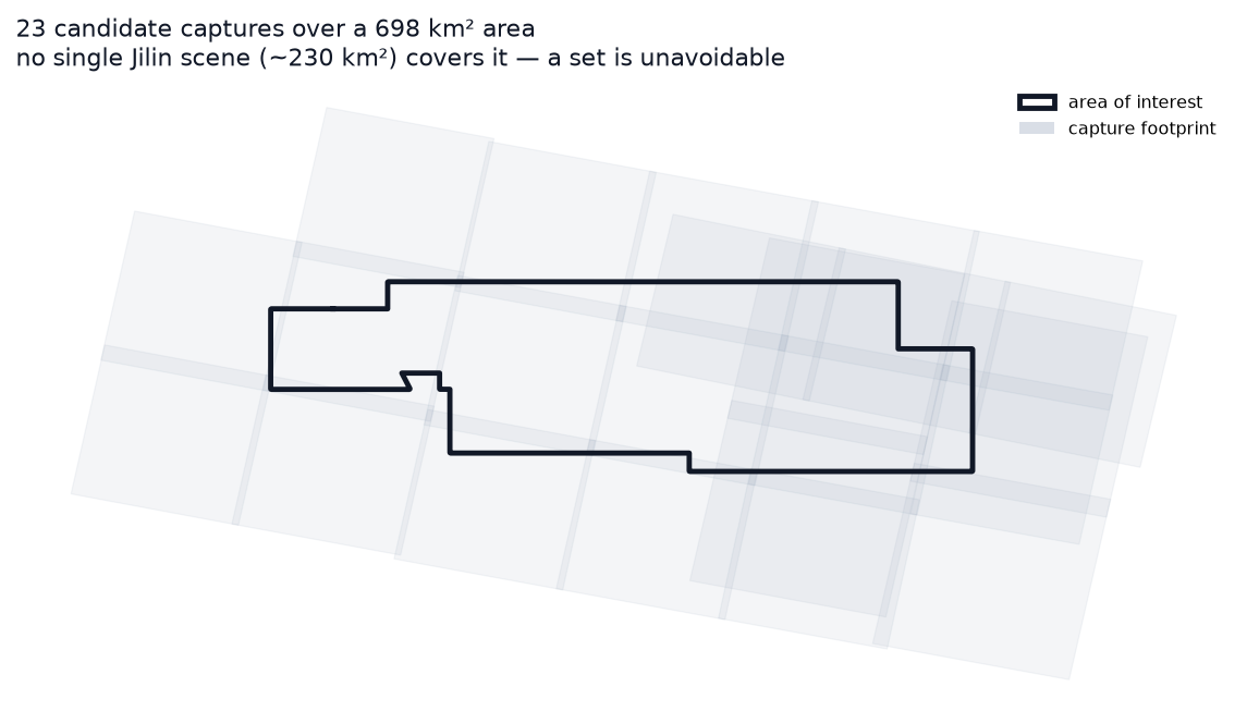
No single footprint covers it. That is not a cloud problem, it is arithmetic — the area is three times a single scene.
What each capture actually delivers
Every one of those 23 captures is reported at 0–1% cloud, and that is correct. Here is what each one delivers over this particular area:
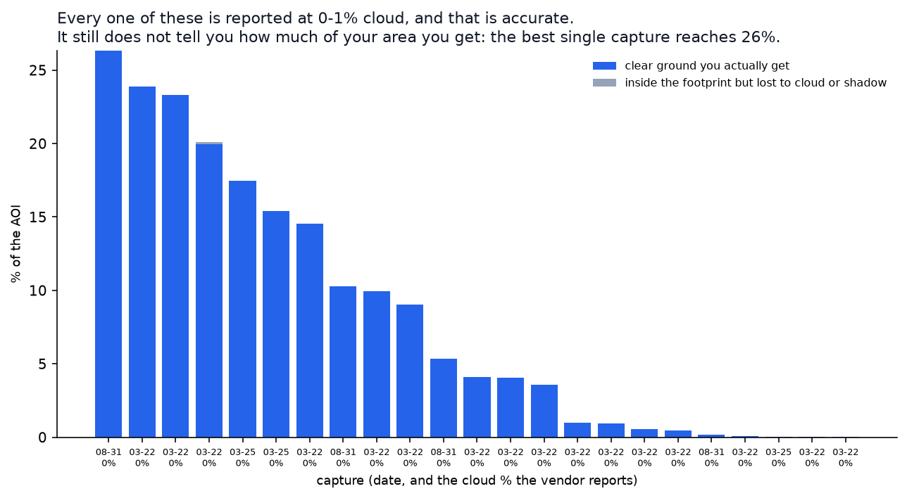
The grey band — ground inside the footprint but lost to cloud or shadow — is barely visible. On this area the vendor’s figure is accurate and the shortfall is almost entirely footprint reach. The best single capture reaches 26.3% of the area.
That distinction is worth keeping straight. The measurement is not usually catching the vendor out on cloud; it is answering a question the vendor’s number does not address — how much of my area do I actually get? When cloud is present it is subtracted; when it isn’t, the measurement says so.
What the planner selected
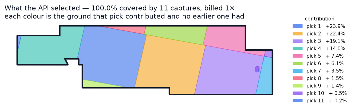
11 captures, 100.0% of the area covered, billed 1×.
| Pick | Date | On its own | New ground added |
|---|---|---|---|
| 1 | 2025-03-22 | 23.9% | +23.9% |
| 2 | 2025-03-22 | 23.3% | +22.4% |
| 3 | 2025-03-22 | 19.9% | +19.1% |
| 4 | 2025-03-22 | 14.5% | +14.0% |
| 5 | 2025-03-22 | 9.9% | +7.4% |
| 6 | 2025-03-22 | 9.0% | +6.1% |
| 7 | 2025-03-22 | 4.1% | +3.5% |
| 8 | 2025-03-22 | 4.0% | +1.5% |
| 9 | 2025-03-22 | 3.6% | +1.4% |
| 10 | 2025-03-25 | 15.4% | +0.5% |
| 11 | 2025-03-22 | 0.5% | +0.2% |
Two things there are the point of the operation.
It did not take the best capture. The single best capture over this area came from a different date entirely, at 26.3%. The planner chose captures that complement each other instead — a set that tiles the area beats a better individual capture that leaves three quarters of it uncovered.
Look at picks 9–11. They add 1.4%, 0.5% and 0.2%. Individually trivial, and a selector optimising for a tidy result would skip them. They are taken because completing the area costs nothing here: summed overlap ends at 1.28×, well inside the 1× band. The last two percent of an area you are paying for is not a rounding error — it is ground you would otherwise have to chase in a second order.
span_days came back 2. Ten of the eleven are from one day and one is three days
later, so this is effectively a mosaic rather than a temporal composite. The response
reports is_composite: true (more than one capture) alongside span_days: 2 — those
answer different questions. Use span_days to judge whether a result is defensible as
a single observation, and max_span_days to constrain it.
What it costs
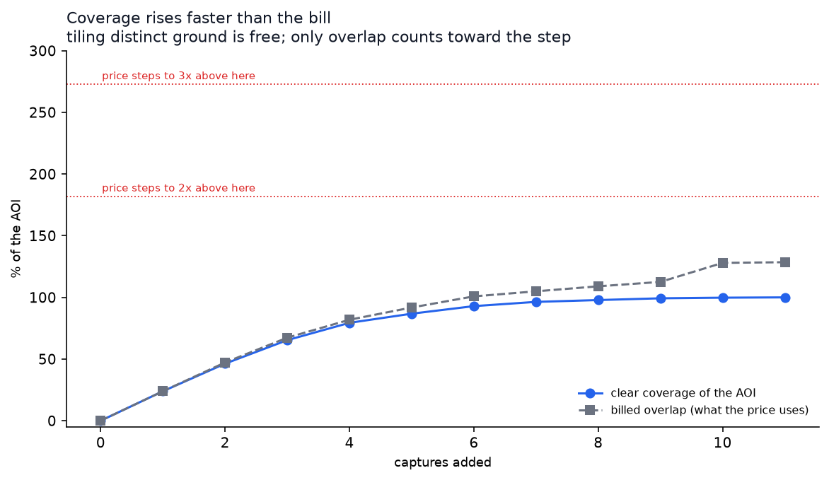
Archive is billed on summed overlap, not on the number of captures and not on a deduplicated union:
coverage_ratio      = Σ(each capture's overlap with the AOI) / AOI area
coverage_multiplier = max(1, floor(coverage_ratio × 1.1))
chargeable_area     = base_chargeable_area × coverage_multiplier
which makes the bill a step function:
| Summed overlap | Billed |
|---|---|
| up to 1.819× | 1× |
| 1.819× – 2.728× | 2× |
| 2.728× – 3.637× | 3× |
Eleven captures tiling this area sum to 1.28× overlap, so it bills 1× — the same as ordering one capture. There is still 0.53× of the area available at no extra cost before the price moves.
That is the counter-intuitive part: tiling distinct ground is free. Only overlap pushes the ratio up. A set that covers your area once, in pieces, costs what a single capture covering it once would cost.
The planner accounts for this. Crossing a threshold is priced as roughly one whole extra cover of the area, and a capture may only push you across one if it adds at least 15% coverage. Without that rule a coverage-maximising selector would double your bill for two more percent of ground.
Calling it
1. Search — no cloud filter
catalog.search is per-host and STAC-shaped. Fan out across hosts yourself, or use catalog.search_stream, which does it for you and emits NDJSON.
curl -s -X POST https://api.geopera.com/v1/op/catalog.search \
  -H "Authorization: Bearer $TOKEN" \
  -H "Content-Type: application/json" \
  -d '{
    "host_name": "the-host",
    "intersects": { "type": "Polygon", "coordinates": [[ ... ]] },
    "datetime": "2025-01-01T00:00:00Z/2025-12-31T23:59:59Z",
    "limit": 200,
    "query": { "cloudCoverage": { "LTE": 100 } }
  }'
The response is a STAC FeatureCollection. Map each feature into a plan scene:
plan field | From the STAC feature |
|---|---|
scene_id | id |
footprint | geometry |
thumbnail_url | properties.thumbnailUrl ?? assets.thumbnail.href |
captured_at | properties.datetime |
off_nadir_deg | properties["view:off_nadir"] |
sun_elevation_deg | properties["view:sun_elevation"] |
vendor_cloud_pct | properties.cloudCoverage ?? properties["eo:cloud_cover"] |
vendor | the host you queried, upper-cased |
A candidate with no browse image cannot be measured. The planner counts it as
contributing nothing rather than assuming it is clear, so drop those before sending.
A single plan call accepts up to 10,000 candidate scenes.
2. Plan
curl -s -X POST https://api.geopera.com/v1/op/catalog.clear_coverage.plan \
  -H "Authorization: Bearer $TOKEN" \
  -H "Content-Type: application/json" \
  -d '{
    "aoi": { "type": "Polygon", "coordinates": [[ ... ]] },
    "scenes": [ { "scene_id": "...", "footprint": { ... },
                  "thumbnail_url": "https://.../browse.jpg",
                  "captured_at": "2025-03-22T02:11:04Z",
                  "vendor": "THE-VENDOR", "vendor_cloud_pct": 0,
                  "off_nadir_deg": 1.4, "sun_elevation_deg": 52.3 } ],
    "max_span_days": 45
}'{
"coverage": 1.0,
"complete": true,
"is_composite": true,
"span_days": 2,
"members": [
{
"scene_id": "...",
"captured_at": "2025-03-22T02:11:04+00:00",
"standalone_clear": 0.2394,
"marginal_gain": 0.2394,
"billed_overlap": 0.2394,
"contribution": { "type": "Polygon", "coordinates": [] }
}
],
"uncovered": null,
"coverage_ratio": 1.28,
"billed_multiplier": 1,
"free_budget_remaining": 0.53,
"needs_review": false,
"review_reason": null,
"excluded_by_filter": {},
"scenes": [{ "scene_id": "...", "clear_fraction": 0.2632 }]
}contribution is the geometry each pick added that no earlier pick had — the coloured
shapes in the figure above. Render it directly rather than recomputing
clear-minus-covered; a second implementation of that arithmetic drifts from the
numbers beside it.
3. Preview the price
curl -s -X POST https://api.geopera.com/v1/op/orders.archive.estimate \
  -H "Authorization: Bearer $TOKEN" \
  -H "Content-Type: application/json" \
  -d '{
    "captures": [
      {
        "id": "...",
        "vendor": "THE-VENDOR",
        "geometry": { "the capture footprint": "from the STAC feature" },
        "maxGSD": 0.75,
        "AOI": { "id": "my-area-1", "geometry": { "your area": "..." } }
      }
    ]
  }'
Each capture needs its id, vendor, footprint geometry, and maxGSD (from the
STAC feature’s properties.gsd). AOI is an object with an id and a geometry, not a bare geometry — the id is yours, and it is how the response
attributes area back to each of your areas when one order covers several. A capture
that cannot be priced comes back in errors with its input index and a reason,
rather than failing the whole request.
Worth doing rather than trusting the plan. plan predicts the price so it can avoid
expensive choices, but estimate is the pricing engine, including contracted
rates and minimum-area rules the planner does not model. Each returned group carries
the coverageMultiplier actually applied — cross-check it against billed_multiplier. They should agree; estimate wins if they ever don’t.
4. Order
curl -s -X POST https://api.geopera.com/v1/op/orders.archive.place \
  -H "Authorization: Bearer $TOKEN" \
  -H "Content-Type: application/json" \
  -d '{ "captures": [ ], "projectId": "...", "licenseType": "..." }'
The same operation covered in Ordering archive imagery. A planned order and a hand-picked one take an identical path — pricing, approval and delivery included.
Request parameters
| Field | Default | What it does |
|---|---|---|
target_coverage | 1.0 | How much of the area to cover. Defaults to all of it: coverage is capped by what the archive holds, so this is an instruction to keep going while progress is available, not a promise. Lower it to stop early — the biggest cost lever, since the last capture is the one most likely to cross a threshold. |
max_span_days | 45 | Hard limit on the date range of a set. 0 forbids combining dates. Not a preference: a set spanning months is not a single observation. |
max_scenes | 20 | Safety ceiling, not a tuning knob — the selection stops on its own when no ground is left worth covering. Lower it if you want to cap the number of separate deliveries. |
target_date | — | Prefer captures near this date. A preference inside your search window, not a filter. |
date_priority | balanced | How hard to pull toward target_date. off; balanced breaks ties without buying a worse capture; strict outweighs even a billing threshold. |
max_off_nadir_deg | — | Hard limit. Off-nadir is already priced, but a preference cannot express never — priced alone, an oblique capture is still chosen if it is the only cover. |
min_sun_elevation_deg | — | Hard limit, same reasoning. |
vendors | — | Restrict to these providers. Absolute, never a ranking: a substitute is not offered even when it is the only capture covering the area. |
min_marginal_gain | 0.001 | Smallest share of the area a capture must add to be taken when taking it is free (it does not raise the multiplier). Raise it if a delivery for 0.1% of ground is not worth the handling to you. |
allow_billing_step | true | Whether any capture may push the order into a higher billing multiplier at all. false caps the order at its current multiplier — a hard price ceiling, at the cost of whatever coverage sat beyond it. |
billing_step_min_gain | 0.15 | How much a capture must add before it is allowed to cross a billing threshold. The guard against buying 2% more ground for twice the price. |
The three threshold parameters exist because the right values depend on what the imagery is for — and a constant you cannot see is a constant you cannot reason about when a result surprises you. The defaults are the behaviour described in this guide.
Anything a hard limit removes is reported in excluded_by_filter, by reason. That
matters — “the archive has nothing here” and “your off-nadir limit rejected all 40
candidates” are indistinguishable otherwise and call for opposite responses.
How selection works
Greedy weighted set-cover over clear-area polygons. At each step it takes the candidate maximising
(new clear ground it adds) / (its marginal cost)stopping when target_coverage is reached or nothing is left worth adding. How much
is “worth adding” depends on the price: a capture that does not push the order into a
higher multiplier costs nothing, so it only has to contribute 0.1% of the area to be
taken. One that would cross a threshold has to earn it — see below.
Greedy is the right tool: it is (1 + ln n)-approximate for set cover, n is 40–100
candidates, and an exact solver would buy a few percent of coverage for an unbounded
worst case across thousands of areas.
Marginal cost blends a small per-capture penalty, off-nadir, low sun elevation,
distance from target_date when you set one, and the billing threshold — priced at
roughly one whole extra cover of the area.
Cloud geometry comes from the vendor’s browse image: it is mapped onto the capture’s footprint, cloud and shadow are segmented from it, and
clear = footprint − cloud − shadow ∩ your AOIA capture whose browse image cannot be read contributes nothing. It is never
assumed clear — unknown ground sold as clear is the failure this exists to prevent.
Such an area returns needs_review: true with a reason.
Cloud-geometry measurement is supported for a subset of providers today; others are
declined by name with a reason rather than silently mis-measured. excluded_by_filter and review_reason tell you which.
Scaling to thousands of areas
What actually costs anything
Measured on the example above: 23 browse images analysed in ~10 s, cold, including fetching each from the vendor. Selection itself is negligible.
So the cost is browse-image analysis, and the thing that controls it is that cloud geometry is a property of a scene, not of an area–scene pair. One footprint covers ~230 km² and will be a candidate for many nearby areas, so results are cached per scene and reused:
3,000 areas × 4 windows × ~40 candidates  =  480,000 analyses   uncached
with ~8 areas sharing each scene          =   60,000 analyses   cached
A cold analysis is ~0.4 s including fetch; a cache hit is ~0.01 s.
Structuring the run
- Search once per area across your whole horizon, not once per area–window. Eight
areas over a year is 8 searches, not 32;
campaignslices the pool per window. - Bound your concurrency. Provider catalogue and asset hosts are shared resources — 4–8 requests in flight is plenty, and the cache absorbs the rest.
- Plan per area, then order in whatever batches suit your workflow.
import asyncio, httpx

BASE, TOKEN = "https://api.geopera.com", "..."
HEADERS = {"Authorization": f"Bearer {TOKEN}"}
SEM = asyncio.Semaphore(6)


async def plan_one(client, aoi, window, target_date=None):
    async with SEM:
        found = await client.post(f"{BASE}/v1/op/catalog.search", headers=HEADERS, json={
            "host_name": "the-host",
            "intersects": aoi["geometry"],
            "datetime": f"{window[0]}/{window[1]}",
            "limit": 200,
            "query": {"cloudCoverage": {"LTE": 100}},   # deliberately unfiltered
        })
        found.raise_for_status()

        scenes = [{
            "scene_id": f["id"],
            "footprint": f["geometry"],
            "thumbnail_url": (f["properties"].get("thumbnailUrl")
                              or f.get("assets", {}).get("thumbnail", {}).get("href")),
            "captured_at": f["properties"].get("datetime"),
            "off_nadir_deg": f["properties"].get("view:off_nadir"),
            "sun_elevation_deg": f["properties"].get("view:sun_elevation"),
            "vendor_cloud_pct": (f["properties"].get("cloudCoverage")
                                 or f["properties"].get("eo:cloud_cover")),
        } for f in found.json().get("features", [])]

        scenes = [s for s in scenes if s["thumbnail_url"]]   # unmeasurable otherwise
        if not scenes:
            return {"aoi_id": aoi["id"], "outcome": "nothing_available"}

        planned = await client.post(
            f"{BASE}/v1/op/catalog.clear_coverage.plan", headers=HEADERS,
            json={"aoi": aoi["geometry"], "scenes": scenes,
                  "max_span_days": 45, "target_date": target_date},
            timeout=180.0)
        planned.raise_for_status()
        return {"aoi_id": aoi["id"], **planned.json()}


async def main(aois, window):
    async with httpx.AsyncClient(timeout=180.0) as client:
        results = await asyncio.gather(
            *(plan_one(client, a, window) for a in aois), return_exceptions=True)

    ready, review = [], []
    for r in results:
        if isinstance(r, Exception):
            continue
        # Never auto-order something the planner does not vouch for.
        (review if r.get("needs_review") or not r.get("complete") else ready).append(r)
    return ready, review
Two habits matter at this scale, both visible above: drop candidates with no browse
image rather than letting them silently contribute nothing, and route needs_review or complete: false to a human instead of ordering them. At 3,000 areas a 2% review
rate is 60 areas — small enough to inspect, large enough to matter if you don’t.
The portfolio question
catalog.clear_coverage.campaign takes many areas and many windows at once and
returns a cell per (area, window) — single_capture, set_of_captures, incomplete or nothing_available — plus the window in which the largest share of your portfolio
is obtainable.
{
	"aois": [{ "aoi_id": "...", "geometry": {} }],
	"epochs": [{ "label": "2026-Q1", "start": "2026-01-01", "end": "2026-03-31" }],
	"scenes": []
}
Within each window it prefers captures near that window’s midpoint — “2026-Q1” means the quarter, and a 1 January capture is not an equally good representative of it as one from mid-February.
This operation is synchronous and capped at 40 areas per call. Chunk beyond that.
Availability is a real constraint — check it first
Measured across 20 areas over a year: one capture reached ≥99% coverage in 21% of windows, a set in 73%. But some months yield nothing at all: in one region, four separate months returned zero captures across every area.
No amount of selection fixes an empty archive. Run campaign before committing to a
quarterly schedule, so an unachievable quarter is a known fact rather than a discovery
halfway through.
Things worth knowing
Areas must be in WGS84 longitude/latitude. GeoJSON requires it (RFC 7946 §4). Projected coordinates — UTM eastings and northings — are rejected, because every intersection, area figure and price derived from them would be meaningless. If you are exporting from a GIS, reproject to EPSG:4326 first.
complete: false is not a failure. It means the archive could not cover your area
to your target, and uncovered is the geometry it could not reach. Decide whether to
lower target_coverage, widen the window, or wait.
Check needs_review. It is set when the planner does not trust its own answer.
Do not auto-order those.
is_composite and span_days answer different questions — more than one capture,
versus how far apart they are.
Distinguish “nothing available” from “your filters rejected everything.” Read excluded_by_filter before concluding the archive is empty.
Related
- Ordering archive imagery — the single-area flow, license types and billing modes.
- Catalog discovery — searching hosts, collections and STAC filters in depth.
- Billing & credits — how chargeable area and credits work.